
 rgpot
Scan a potential energy surface over RPC
This tutorial sends geometries to the rgpot server over remote procedure calls (RPC) and draws what comes back. You will evaluate one Lennard-Jones (LJ) pair, scan the energy curve of two pair potentials and check their forces, then map a two-dimensional surface for a hydrogen molecule above a copper slab with an embedded-atom method (EAM) potential. The end result is the two figures on this page, made on your machine.
What you will need
The build from the Quickstart:
bbdir/CppCore/potservfrommeson setup bbdir -Dwith_tests=true -Dwith_rpc=true.The
rpctestshell from the same page (pixi shell -e rpctest), which providespycapnp,numpy,scipyandmatplotlib.
Run every command from the repository root.
Step 1: start a server
potserv takes a port and the name of one potential:
./bbdir/CppCore/potserv 12345 LJ &
It prints Loading LJ potential... and then
Server running on port 12345 with LJ potential. when it is ready.
Step 2: send one geometry
The client below is the whole conversation.
It loads the schema, connects, fills one ForceInput with positions, atomic
numbers and the cell, and reads energy and forces from the PotentialResult.
"""Send one geometry to a running potserv and print the reply.

    ./bbdir/CppCore/potserv 12345 LJ
    python docs/orgmode/tutorials/pes_scan/evaluate_once.py 12345
"""

import asyncio
import sys
from pathlib import Path

import capnp
import numpy as np

ROOT = Path(__file__).resolve().parents[4]
schema = capnp.load(str(ROOT / "CppCore/rgpot/rpc/Potentials.capnp"))


async def connect(port):
    """Return a client for the Potential interface served on port."""
    for _ in range(100):
        try:
            stream = await capnp.AsyncIoStream.create_connection(host="localhost", port=port)
            client = capnp.TwoPartyClient(stream)
            return client, client.bootstrap().cast_as(schema.Potential)
        except OSError:
            await asyncio.sleep(0.05)
    raise ConnectionError(f"nothing is listening on port {port}")


async def calculate(potential, positions, numbers, box):
    """Send one geometry; return the energy and an (N, 3) force array."""
    request = schema.ForceInput.new_message()
    request.pos = np.ravel(positions).tolist()
    request.atmnrs = list(numbers)
    request.box = np.ravel(box).tolist()
    reply = await potential.calculate(request)
    return reply.result.energy, np.reshape(reply.result.forces, (-1, 3))


async def main(port):
    _client, potential = await connect(port)
    positions = [[0.0, 0.0, 0.0], [1.2, 0.0, 0.0]]
    energy, forces = await calculate(potential, positions, [0, 0], 20.0 * np.eye(3))
    print(f"energy: {energy:.6f} eV")
    for i, f in enumerate(forces):
        print(f"force on atom {i}: [{f[0]:+.6f}, {f[1]:+.6f}, {f[2]:+.6f}] eV/Angstrom")


if __name__ == "__main__":
    asyncio.run(capnp.run(main(int(sys.argv[1]) if len(sys.argv) > 1 else 12345)))
python docs/orgmode/tutorials/pes_scan/evaluate_once.py 12345
energy: -0.890965 eV
force on atom 0: [+2.211693, +0.000000, +0.000000] eV/Angstrom
force on atom 1: [-2.211693, +0.000000, +0.000000] eV/Angstrom
The built-in LJ potential has a well depth of 1 eV and a zero crossing at 1
Angstrom (CppCore/rgpot/LennardJones/LJPot.hpp).
At 1.2 Angstrom the pair sits outside its minimum, so each atom is pulled toward
the other and the two forces are equal and opposite.
Stop the server before the next step:
kill %1
Step 3: scan two pair curves and check the forces
scan_pes.py starts its own potserv for each potential, sends one geometry
per call over a single connection, and stops the server when the scan ends.
It reuses connect and calculate from the client above.
python docs/orgmode/tutorials/pes_scan/scan_pes.py --server-bin ./bbdir/CppCore/potserv
The script writes dimer_curves.png and cuh2_elbow.png into
docs/orgmode/tutorials/pes_scan/, over the copies in the repository.
The first lines of output cover the two pair potentials:
LJ dimer: 200 distances from 0.95 to 3.00 Angstrom
  lowest energy -0.999800 eV at r = 1.1251 Angstrom
  largest |force - (-dE/dr)| = 2.79e-07 eV/Angstrom
Morse dimer: 200 distances from 2.30 to 7.00 Angstrom
  lowest energy -0.710085 eV at r = 2.8905 Angstrom
  largest |force - (-dE/dr)| = 2.43e-09 eV/Angstrom
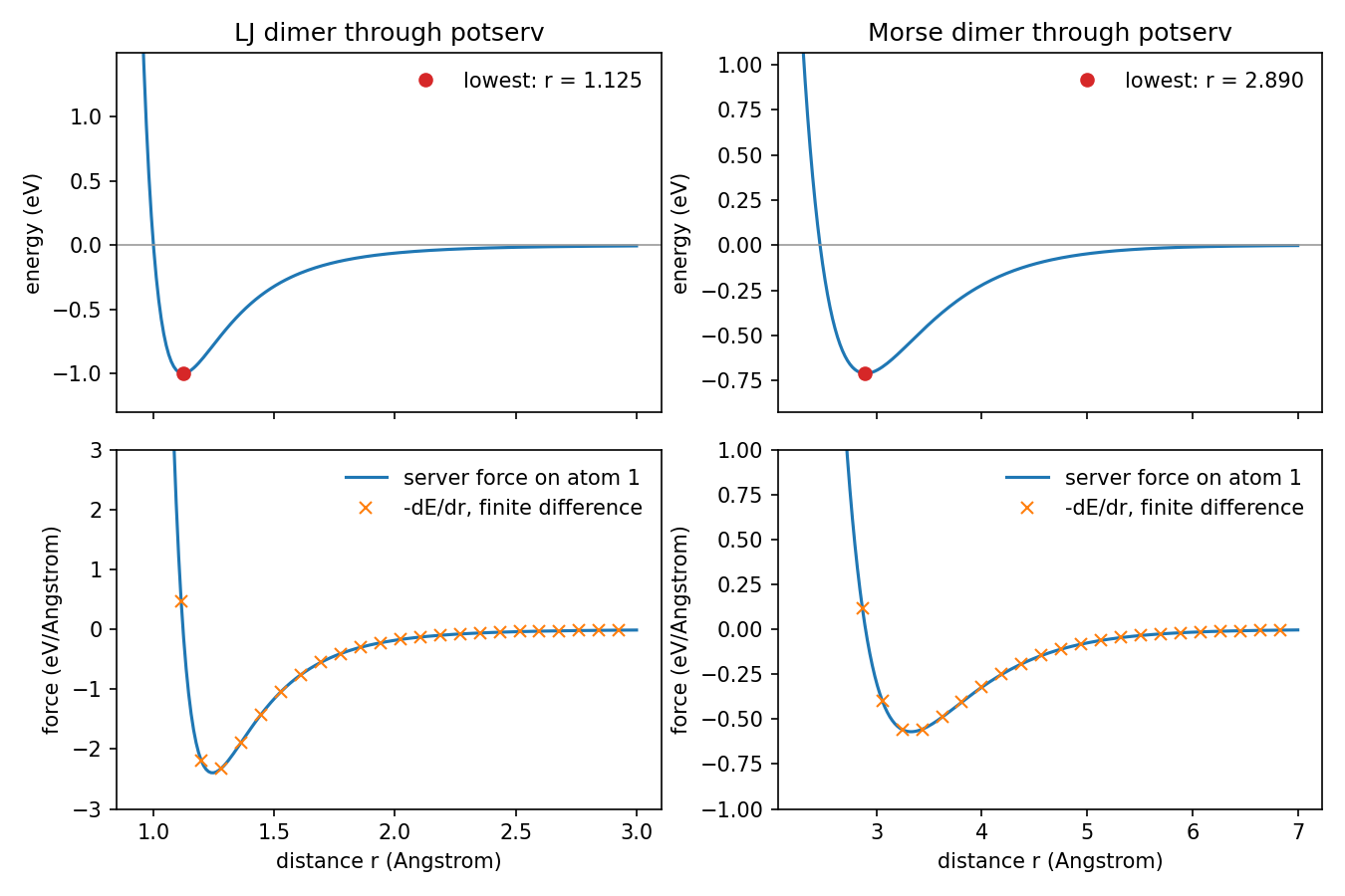
Energy (top) and force on the second atom (bottom) for an LJ pair and a Morse pair, each evaluated through potserv. Crosses are minus the central difference of the energy, step 1e-5 Angstrom.
The lowest LJ grid point is the one nearest the 12-6 minimum, which sits at the
sixth root of 2 times the zero crossing (1.1225 Angstrom).
The Morse server uses platinum parameters, a well depth of 0.7102 eV at 2.8970
Angstrom (CppCore/rgpot/Morse/MorsePot.hpp); its lowest grid point is
-0.710085 eV at 2.8905 Angstrom.
The force check is the useful habit: the force the server returns should be
minus the slope of the energy it returns.
Here the two agree to 2.79e-07 eV/Angstrom for LJ and 2.43e-09 eV/Angstrom for
Morse.
The error of a central difference grows with the step squared times the third
derivative, which is largest at the LJ repulsive wall, so these gaps measure the
check rather than the server.
Step 4: map a surface with the copper-hydrogen EAM
The same script then loads the Cu slab from CppCore/rgpot/CuH2/tmp.con, puts
an H2 molecule above it, and varies two numbers: the H-H bond length and the
height of the molecule’s centre above the top copper layer.
The molecule keeps the lateral position and orientation of the H2 in that file.
The reference energy is the same slab with the molecule 50 Angstrom up, beyond
the 6.1 Angstrom cutoff of the potential
(CppCore/rgpot/fortran/rgpot_cuh2.f90).
fixture H2: bond 1.3428 Angstrom, height 0.8520 Angstrom
CuH2 elbow: 4158 geometries of 216 Cu + 2 H
  top Cu layer z = 6.9835 Angstrom, H2 centre x, y = 8.3122, 9.9470
  gas-phase H2, 50 Angstrom up: -697.291025 eV at bond 0.7200 Angstrom
  molecule: +0.0085 eV at bond 0.7600, height 3.5000 Angstrom
  atoms apart: +0.2127 eV at bond 3.0000, height 0.8000 Angstrom
  lowest ridge between them on this grid: +0.6785 eV
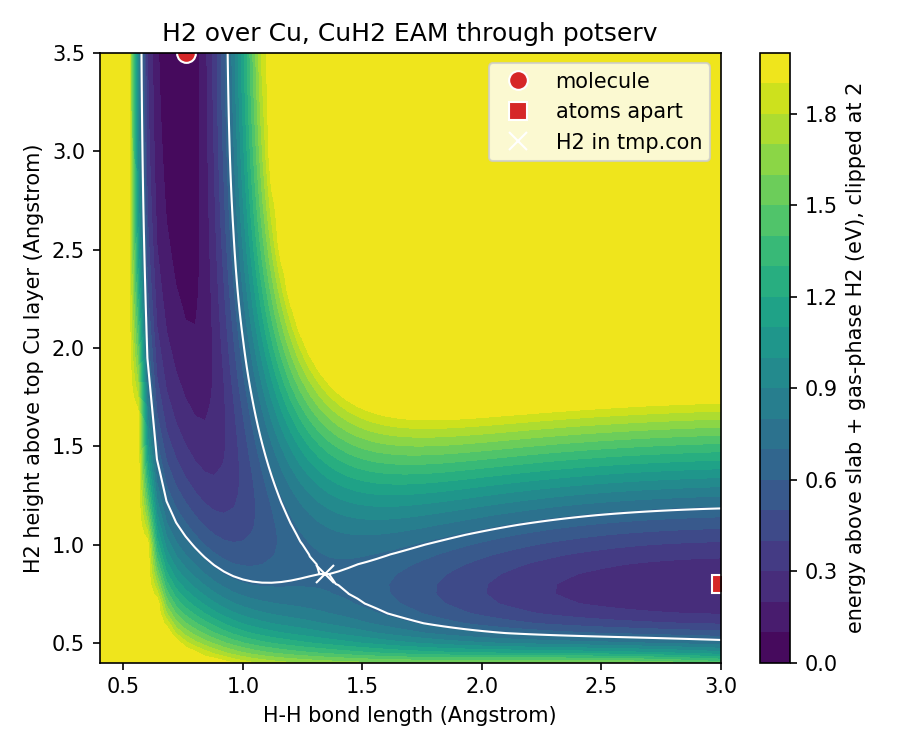
Energy of H2 above the Cu slab relative to the slab plus a distant H2, on a grid of 4158 geometries. The white contour is the lowest level that joins the molecule channel (circle) to the dissociated channel (square); the cross is the H2 geometry stored in tmp.con.
Read the map as two valleys.
The upper left valley is the intact molecule far from the surface.
The lower right valley is the two hydrogen atoms apart, close to the copper; it
sits 0.2127 eV above the gas-phase molecule at the edge of the grid.
To get from one valley to the other the molecule has to cross a ridge, 0.6785 eV
on this grid, where the white contours meet.
The H2 stored in tmp.con (the cross) sits at that crossing.
What just happened
Every energy and force on this page came from potserv over Cap’n Proto RPC.
The client sent a ForceInput per geometry and read back a PotentialResult;
it never linked against the potential code.
Swapping LJ for Morse or CuH2 changed only the name given to the server.
Any other selector the server was built with, such as an extended tight-binding
(xTB) or metatomic model, answers the same client.
The RPC Model explains why the wire is split this way
and draws the client, server and backend layout.
Next steps
External Integration Guide: call the same server from C++.
Find the Ground State of an EON Structure: drive the server from Atomic Simulation Environment (ASE) optimizers.
Saddle searches on this stack, with eOn driving a potential that rgpot serves over RPC: Goswami, Gunde and Jónsson, Frontiers in Chemistry (2026), https://doi.org/10.3389/fchem.2026.1807063.
The Morse potential is from Morse, Physical Review 34, 57 (1929), https://doi.org/10.1103/PhysRev.34.57.
The 12-6 form is from Lennard-Jones, Proceedings of the Royal Society A 106, 463 (1924), https://doi.org/10.1098/rspa.1924.0082.